5.7.2 Prediction and residual values

When running binary regression analyzes through the logit or probit commands, there are two ways to extract prediction values. One way is through the use of the command logit-predict or probit-predict which can be used to generate a new variable with individual prediction values, probability values ​​or residual values ​​(not probit-predict). These can be used for further input for various statistical purposes. The second way is to use the margins() option, which returns a fully calculated prediction value for the response variable measured by the average of all explanatory variables included.

Generate new variable with individual prediction, probability or residual values

All regression variants found in microdata.no have associated commands that generate, among other things, residual and prediction values. These are values ​​that can be used to analyze the data spread and for testing regression models. Prediction values ​​can also be used as input for further analyses.

The commands have the same name as the corresponding regression command plus -predict.

Syntax:

 logit-predict <variable> <variable list> [if <condition>] [,<options>]

 probit-predict <variable> <variable list> [if <condition>] [, <options>]

The variables are entered in the same way as for the corresponding regression model which is run with the command logit or probit.

The following values ​​can be retrieved:

• logit-predict: Probability values, prediction values ​​and residuals

• probit-predict: Probability values ​​and prediction values

You decide for yourself which values ​​you want to generate through the use of options. The result of the runs is a set of variables that contain the various values. By default, the first-mentioned value type is generated in the list above, but it is still recommended to specify this through options, as you can then also determine the name of the generated variables inside a parenthesis as shown in the syntax example below. If you run several -predict commands, you must create new names for them automatically generated the variables.

Syntax example:

 logit-predict high salary age male wealth, residuals(res4) predicted(pred4) probabilities(prob4)

The automatically generated variables can be used as input for further analyzes or to be displayed graphically. Current graphical commands are hexbin and histogram. By running histogram on the residual variable, you can check whether the residuals are normally distributed. The hexbin command can also be used to create anonymized scatterplots where two sets of values ​​are combined.

For more details, it is recommended to use the command help logit-predict or help probit-predict.

 $\rhd$ Example: Prediction and residual values analysis

Calculate predicted value for response variable measured by the average of the explanatory variables

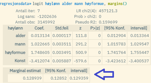
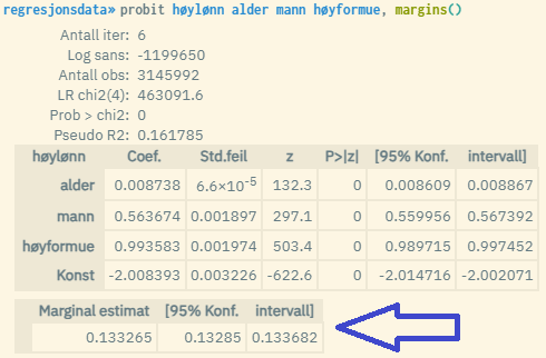
By using the margins() option when running binary/logarithmic regression models through the logit or probit commands, you can easily find the fully calculated predicted value for the response variable (Y) measured by the mean value for all the respective explanatory variables.

Examples:

What is then returned under the model estimates is the predicted Y-value and the confidence interval. "Marginal estimate" (so predicted Y) can be interpreted as "expected value of Y measured for an average person", and is based on a standard calculation where each of the estimated coefficient values ​​is multiplied by the average value for the associated explanatory variable (x). These are then summed together with the constant term in line with the estimated regression equation:

  $\hat{Y} = const + b_1 \bar{x_1} + … + b_n \bar{x_n}$

Note that with logarithmic models given by logit and probit, the coefficient estimates b cannot be interpreted as marginal effects in the same way as for regression. Predicate Y is therefore based on the following transformation:

• logit: $\hat{Y} = 1 / (1 + e^{-\hat{Y}})$

• probit: $\hat{Y} = \Phi(\hat{Y})$

(Note: $\Phi()$ is the cumulative normal distribution function)

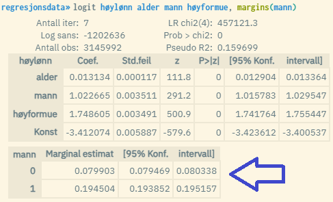
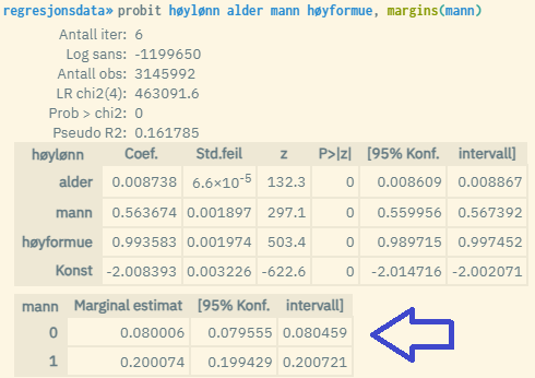
You can also enter a dummy variable inside the parentheses in margins(). Then you will get two extra lines returned under the model estimates, i.e. predicted Y value for each value of the dummy variable (values ​​0 and 1). You then estimate predicted Y for each of the two groups with the value 0 and 1, where all other explanatory variables are measured at the average value. Note that the dummy variable you use must also be included in the regression model itself. In practice, the "expected value of Y for an average person in the respective groups 0 and 1" is then estimated. If you e.g. using the dummy variable "man", then one measures the expected value of Y for an average man and an average woman.

Examples:

Note that when calculating predicted Y values, the Winsorized average is used, i.e. an average that could potentially be affected by winsorization of extreme values. In practice, this means that the average values ​​used in the calculations of predicted values ​​are somewhat lower than the actual values ​​in some cases. You can read more about winsorisation here: https://microdata.no/manual/konfidensialitet#tiltak-2-winsorisering

Unlike logit-predict and probit-predict which generate a dataset of predicted values ​​for each unit given the actual values ​​of the explanatory variables, the margins option calculates predicted Y values ​​measured by the mean of the respective explanatory variables measured over the entire population. Therefore, when using the summarize command to show the average predicted Y value based on the dataset of individual predicted values ​​generated through the -predict commands, these will not match the values ​​reported through the margins option.

 $\rhd$ Example: Find prediction value for the response variable